
Data tables in the form of spreadsheets are ubiquitous in enterprise. For better or worse, they are the Swiss Army Knife (or cockroaches) for decision support in many organisations.
Why are they so popular and widely used? That’s not the focus of this blog, instead we focus on how you might go about automating the classification of spreadsheets without manually having to open and inspect them. We use some of the techniques we used in previous posts to represent a spreadsheet as a matrix (empty or not-empty cells) and attempt dimension reduction. We also focus on feature extraction of spreadsheets by reviewing the literature and drawing from the experience of experts who do PhDs on this sort of thing.
In this post we refer to workbooks as spreadsheets and worksheets as sheets.
The problem
Tabular data is an abundant source of information on the internet, but remains mostly isolated from the latter’s interconnections since spreadsheets lack machine readable descriptions of their structure. The structure can be widely varied and inconsistent, written for human interpret-ability foremost.
Most organisations have an abundance of spreadsheets, too many to sort and label manually, often stored in a jumble of directories. Too many to quality assure retrospectively. An automated method for labeling spreadsheets could help with knowledge management and searching for relevant spreadsheets to address business needs as well as identifying areas of business risk. As well as classifying the general content of a spreadsheet (such as the classic case study of 16,189 Enron spreadsheets), perhaps this approach could be used to identify those spreadsheets that have a nice or tidy structure or contain sensitive information. These could be useful tags or classification by theme for an organisation to have on it’s spreadsheets, such as spreadsheets found at data.gov.uk / gov.uk (credit to Duncan Garmonsway for this idea).
The following framework can be used to approach this problem:
- select labelled spreadsheets to train classification algorithms
- preprocess the data and extract features
- train the algorithm
- evaluate the derived model on test spreadsheets
- classify new spreadsheets
Thinking about spreadsheet features
Spreadsheets consist of textual values in a two-dimensional grid format. They are popular precisely because of their high information density due to the semantic meaning communicated in their layout and structure. Often this may be implicit and learned by spreadsheet users as a cultural norm throughout their career and exposure to different conventions. These cultural norms for spreadsheets probably vary from organisation to organisation with some feature being useful regardless of the business. Thus, we might a expect a representative training set to be key to training a good classifier (The famous EUSES spreadsheets are open source and might not be representative of closed source spreadsheets found in an organisation as argued here). We might not expect a model trained on the Enron spreadsheets to perform well on the spreadsheets found on data.gov.uk.
However, these demonstrative examples on model data sets can inform our decision making for feature extraction by standing on the shoulders of giants:
- This ENRON paper also identifies some useful proxy measures of a spreadsheets quality by categorising the “smells” in a spreadsheets formulae (e.g. unique formulas that have a calculation chain of five or longer).
- This could be useful for an organisation attempting to audit the quality of its spreadsheets and flagging spreadsheets for quality assurance.
The data
The data is pretty big (almost 1 Gb zipped) so we don’t store it in our repo. Instead download it from origin at figshare (Hermanns, 2015). Unfortunately this data is in .xlsx format.
Some interesting points about this Enron spreadsheet data, especially if it is representative of other organisations (albeit it is somewhat dated now):
- 24% of Enron spreadsheets with formulas contain an Excel error. It’s also noted that formal testing (software development) is rare in spreadsheets in general, discussed in a recent paper, the very thing required to protect against these errors.
- There is remarkably little diversity in the functions used in spreadsheets: we observe that there is a core set of 15 spreadsheet functions which is used in 76% of spreadsheets. Thus, these could be readily replaced by a software package containing this core set used across the organisation and developed using DevOps best practice. This supports the case for developing reproducible analytical pipelines in an organisation.
- Spreadsheet use within companies is common, with 100 spreadsheets emailed around per day! Version control is essential for collaboration, yet looks like Enron didn’t use it…
Reading the data
We copy and modify Duncan’s code to read in the spreadsheets. It’s great practice to work with another data scientist on a project to help you learn new tips and tricks (for example, I hadn’t seen the here package before).
# Googled it, it's not on CRAN yet
# devtools::install_github("krlmlr/here")
# devtools::install_github("ironholds/piton")
# devtools::install_github("nacnudus/tidyxl")
Workbooks
We look at the spreadsheet files.
c(
  head(list.files("./data/enron_spreadsheets/"), 3),
  tail(list.files("./data/enron_spreadsheets/"), 3)
)
## [1] "albert_meyers__1__1-25act.xlsx"
## [2] "albert_meyers__2__1-29act.xlsx"
## [3] "andrea_ring__10__ENRONGAS(1200).xlsx"
## [4] "vladi_pimenov__41078__vladi.xlsx"
## [5] "vladi_pimenov__41079__DailyPrices.xlsx"
## [6] "vladi_pimenov__41080__Basis Spreads for Mike Grigsby.xlsx"File names presumably have the sender (or receiver prefixed) and are of the .xlsx type, thus we need the tidyxl package to read them in. Some spreadsheets it is possible to guess what the contents might be from title alone, others the theme would only be apparent on opening.
# Set the path to your directory of Enron spreadsheets here
enron_path <- "./data/enron_spreadsheets/"

# Set the sample size for testing here
sample_size <- 100

library(dplyr)
library(purrr)
library(tidyxl)
library(here)
library(readxl)

all_paths <- list.files(enron_path,
                        full.names = TRUE)

# For testing, look at n (sample_size) random workbooks.
set.seed(1337)
sample_paths <- sample(all_paths, sample_size)

paths <- sample_paths
Looking at the length of all_paths suggests almost 16 thousand unique spreadsheets (workbooks) in our directory.
length(all_paths)## [1] 15929Worksheets
In our sample of spreadsheets (100) we see that a spreadsheet can have a number of sheets associated with it. We use purrr to apply a function element-wise to a list. We then unlist and count the number of sheets per workbook and plot as a histogram.
# purr package
# https://jennybc.github.io/purrr-tutorial/index.html
sheet_count <- purrr::map(paths, readxl::excel_sheets) %>%
  purrr::map(length) %>%
  unlist()

hist(sheet_count, main = "")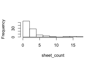
Data range within worksheets
Let’s work out what’s typical in terms of the height (number of rows) and width of a sheet (number of columns) by sampling. We can then set our “view” to encapsulate this typical range (although readxl does this automatically by skipping trailing emp). We need to read the spreadsheets in and look at some features using the readxl package combined with purrr for readability.
To load all the sheets in a workbook into a list of data frames, we need to:
- Get worksheet names as a self-named character vector (these names propagate nicely).
- Use
purrr::map()to iterate sheet reading.
books <-
  dplyr::data_frame(filename = basename(paths),
             path = paths,
             sheet_name = purrr::map(paths, readxl::excel_sheets)
             ) %>%
  dplyr::mutate(id = as.character(row_number()))
We look at one workbook and peek at its first sheet therein.
head(books$sheet_name)## [[1]]
## [1] "MLP's"
##
## [[2]]
## [1] "DJ SP15"
##
## [[3]]
## [1] "newpower-purchase 10'00"
##
## [[4]]
## [1] "value" "positions" "swaps" "Run Query" "Results"
##
## [[5]]
## [1] "MAY-00"
##
## [[6]]
## [1] "EOL"It might be more useful to treat each worksheet as the experimental unit by having one row per worksheet and a list column for the data therein plus extra variables could be added later as we extract features from the worksheets.
Reading data from many workbooks’ many sheets
This was trickier than anticipated as testified by my appeal to help at Stack Overflow. If you want an explanation of the code below, refer to the link above.
First, list the filenames, which will passed to readxl::excel_sheets() for the names of the sheets within each file, and readxl::read_excel() to import the data itself.
library(openxlsx)
library(tidyr) # for unnest to expand a list column

# paths was our sample paths to each of the spreadsheets
x <- tibble::data_frame(path = paths)
Then “Map” the readxl::excel_sheets() function over each of the file paths, and store the results in a new list-column. Each row of the sheet_name column is a vector of sheet names.
x <- dplyr::mutate(x, sheet_name = purrr::map(path, readxl::excel_sheets))We need to pass each filename and each sheet name into readxl::read_excel(path=, sheet=), so the next step is to have a data frame where each row gives a path and one sheet name. This is done using tidyr::unnest().
x <- tidyr::unnest(x)Now each path and sheet name can be passed into readxl::read_excel(), using purrr::map2() rather than purrr::map() because we pass two arguments rather than one.
sheets <- dplyr::mutate(dplyr::slice(x, c(1:10, 12:13, 20:30, 80:100)),
                   data = purrr::map2(path, sheet_name,
                                          ~ readxl::read_excel(.x, .y)))
The reason for the weird slice() is that we have to avoid some worksheets. readxl turns out to have a bug that means it errors on worksheet 14 daren_farmer__6529__egmnom-Jan.xlsx sheet 6 Module1, so the function passed to mutate() will have to cope with errors. The bug is that it expects sheets to have a data file, but it turns out that empty sheets don’t have data files. We can dodge this bug by trial and error so that we get a reasonable sample to work out the typical size of a worksheet.
sheets$sheet_name[3]
str(sheets$data[3])
The dimensions of the data in each sheet is useful for determining its size but note how there are lots of empty cells, including missing rows and columns making it very different to a tidy data frame we would prefer to work with. However, it may serve as a rough proxy for the “area” of cells occupied in a sheet. Thus we count the number of variables and rows to give us the dimensions.
# This doesn't compile properly, so we don't evaluate it here
sheets_data_attr <- lapply(sheets$data, attributes)

df_columns <- purrr::map(sheets_data_attr, "names") %>%
  purrr::map_int(length)

df_rows <- purrr::map(sheets_data_attr, "row.names") %>%
  purrr::map_int(length)

sheets_data_attr %>% {
  tibble::tibble(
       row_dim = df_rows,
    col_dim = df_columns
  )
} -> df

# eyeball and draw a square
plot(y = df$row_dim, x = df$col_dim)
abline(v = 35, h = 85, col = "red")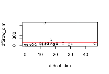
From this plot we eyeball that a rectangle of 35 columns and 85 rows captures approximately 95% of the data in this sample. Typically a spreadsheet has more rows than it does columns; it’s longer than it is wide.
sum((df$row_dim > df$col_dim)) / nrow(df)## [1] 0.8636364We use this information to adjust the view in Duncan’s code (we limit the view range to capture typical spreadsheets and reduce computation).
Limitations
By reading in as a data frame, due to the non-tidy of the worksheets often variables that look like numeric variables will be labelled as chr because of how readxl guesses the column variables based on the first thousand rows (as default). If it contains a mix then often the variable defaults to being described as a character variable in R (demonstrated below; try it yourself).
suppressWarnings(as.numeric("three"))
as.character("three")
as.numeric(3)
as.character(3)
On reading it in, we can only ascertain whether a cell is empty or not (assuming recognised NA placeholders were used in the spreadsheets). We can use this to visualise the shape of the sheet in each spreadsheet workbook and incorporate our learning from the previous section. However, the tidyxl package allows you to extract cell metadata (what’s the contents e.g. formatting and values).
# Set the view range here, described here
view_rows <- 1:85
view_cols <- 1:85  # make it square matrix

# create a row*col cells
view_range <- tidyr::crossing(row = view_rows, col = view_cols)

load_view_range <- function(x) {
  cells <- tidyxl::xlsx_cells(x)
  formats <- tidyxl::xlsx_formats(x)$local
  formatting <-
    data_frame(biu = formats$font$bold
                     | formats$font$italic
                     | !is.na(formats$font$underline),
               fill = !is.na(formats$fill$patternFill$patternType),
               border = !is.na(formats$border$top$style)
                        | !is.na(formats$border$bottom$style)
                        | !is.na(formats$border$left$style)
                        | !is.na(formats$border$right$style),
               indent = formats$alignment$indent != 0L) %>%
    dplyr::mutate(local_format_id = row_number())
  cells %>%
    dplyr::inner_join(view_range, by = c("row", "col")) %>% # filter for the view range
    dplyr::select(sheet, row, col, character, numeric, date, is_blank, local_format_id) %>%
    dplyr::mutate(character = !is.na(character),
           numeric = !is.na(numeric),
           date = !is.na(date)) %>%
    dplyr::left_join(formatting, by = "local_format_id") %>%
    dplyr::select(-local_format_id)
}

view_ranges <-
  map_dfr(books$path, suppressWarnings(load_view_range), .id = "id") %>%
  inner_join(books, by = "id") %>%
  select(-id, -path) %>%
  mutate(biu       = !is_blank & biu,
         fill      = !is_blank & fill,
         border    = !is_blank & border,
         indent    = !is_blank & indent,
         character = !is_blank & character,
         numeric   = !is_blank & numeric,
         date      = !is_blank & date) %>%
  group_by(filename, sheet) %>% # pad each view range with blanks
  tidyr::complete(row = view_rows,
           col = view_cols,
           fill = list(is_blank = TRUE,
                       biu = FALSE,
                       fill = FALSE,
                       border = FALSE,
                       indent = FALSE,
                       character = FALSE,
                       numeric = FALSE,
                       date = FALSE)) %>%
  dplyr::ungroup()

# Check that there is a complete view range for all sheets
nrow(view_ranges) / nrow(view_range) == nrow(distinct(view_ranges, filename, sheet))
We then convert to a wide matrix with each row representing one worksheet and each column a cell.
# Convert to a matrix, one row per sheet, one column per cell
feature_matrix <-
  view_ranges %>%
  dplyr::arrange(filename, sheet, row, col) %>%
  dplyr::rename(y = row, x = col, z = is_blank) %>%
  dplyr::mutate(z = as.integer(z)) %>% # encode blanks as 0
  dplyr::pull(z) %>%
  matrix(ncol = nrow(view_range), byrow = TRUE)
feature_names <-
  view_ranges %>%
  dplyr::distinct(filename, sheet) %>%
  dplyr::arrange(filename, sheet) %>%
  dplyr::mutate(rownames = paste(filename, "|", sheet))
rownames(feature_matrix) <- feature_names$rownames

dim(feature_matrix)
## [1] 262 7225We now have a large matrix which captures the “look” of every spreadsheet. We can visualise this to demonstrate by setting blank cells to beige and cells with contents to red.
# Plot a few of them.  red = value, beige = blank
image_inputs <-
  view_ranges %>%
  dplyr::rename(x = row, y = col, z = is_blank) %>%
  dplyr::mutate(z = as.integer(z)) %>% # encode blanks as 0
  dplyr::group_by(filename, sheet) %>%
  dplyr::arrange(filename, sheet, desc(x), y) %>% # Flip along a horizontal axis for plotting
  dplyr::ungroup() %>%
  tidyr::nest(-filename, -sheet) %>%
  dplyr::mutate(matrix = purrr::map(data,
                                    ~ matrix(.x$z, ncol = length(view_cols)))) %>%
  dplyr::slice(c(8:13))
We slice out some worksheets to visualise, with the workbook name above the image and the worksheet below in grey. Because our view range isn’t square it means it is harder to relate the image to the spreadsheet compared to Duncan’s examples. However, by being more likely to catch most of the data in the worksheet the feature matrix may provide a better representation of the worksheet it represents.
par(mfrow = c(2, 3))

par(adj = 0)
# map over multiple inputs simultaneously
# This syntax allows you to create very compact anonymous functions.
purrr::pwalk(list(image_inputs$matrix, image_inputs$filename, image_inputs$sheet),
      ~ {image(..1, axes = FALSE); title(..2, sub = ..3)})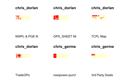
We notice the left-handedness of the images as this matches the typical zoom and opening view when reading the spreadsheets in Excel (one starts in the top left corner; also rows are narrower than columns so you can fit more rows on the screen). Here we see the value of the square matrix for the view_range which gives us an image comparable to the worksheets upon inspection. Some spreadsheets have islands of filled cells far from the main body, this is often some extra annotation or versioning by the author.
t-SNE
Unfortunately we lack a suitable label for the worksheets (i.e. tidy, or contains an error) which means we are in the unenvious position of having to make sense of the spreadsheets using dimension reduction techniques. The plots above are effective when interpreted by a human for getting a sense of the shape of the data in a sheet (and could be extended by using different colours for different cell contents type e.g. formula, error, number etc.) but can we capture the essence of how sheets are filled using dimension reduction techniques? We could then automate our interpretation of a sheet without having to look at it. Useful when most organisations are drowning in spreadsheets.
We plot the row numbers so we can look up and compare the worksheets that are clustered together. Remember with t-SNE, rather than keeping dissimilar data points apart (like linear methods i.e. PCA), t-SNE keeps the low-dimensional representations of very similar data-points close together on a low-dimensional, non-linear manifold (CAVEAT: when using t-SNE in my previous blog post we learnt some important lessons).
Bear in mind if the worksheets by the same author are organised sequentially by row number. Thus we could have used row number as our plotting font to give this extra bit of info, however you’ll need to manually inspect them afterwards to work out why they are close together following t-SNE.
library(Rtsne)
set.seed(2481632)
tsne <- Rtsne(feature_matrix, check_duplicates = FALSE) # Demanding with many sheets

#####------
par(mfrow = c(1, 1))

  plot(tsne$Y,
       # type = "n",
       pch = 21, cex = 0.6,
       main = paste("t-SNE of Enron: in", nrow(books), "books",
                            "and", length(unlist(unique(books$sheet_name))), "worksheets."))
# text(x = tsne$Y[, 1],
#      y = tsne$Y[, 2],
#      labels = seq_along(1:nrow(feature_names)),
#      cex = c(0.5, 0.6, 0.7), # different size to help discern worksheet number
#      col = c("black", "blue", "green"))  # colours to help read worksheet number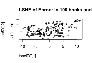
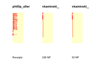
We notice that there are quite a few distinctive high cluster blobs which warrant further inspection. For example, the worksheets to the top-right. Indeed they are close together, possibly by the same author.
w <- which(tsne$Y[, 1] > 9 & tsne$Y[, 2] > 10)
w
paste("There are ", length(w), "worksheets in this range.")
## [1] 80 81 82 83 84 85 86 87 88 89 90 91 92 93 94## [1] "There are 15 worksheets in this range."# Plot a few of them. red = value, beige = blank
image_inputs <-
view_ranges %>%
dplyr::rename(x = row, y = col, z = is_blank) %>%
dplyr::mutate(z = as.integer(z)) %>% # encode blanks as 0
dplyr::group_by(filename, sheet) %>%
dplyr::arrange(filename, sheet, desc(x), y) %>% # Flip along a horizontal axis for plotting
dplyr::ungroup() %>%
tidyr::nest(-filename, -sheet) %>%
dplyr::mutate(matrix = purrr::map(data,
~ matrix(.x$z, ncol = length(view_cols)))) %>%
dplyr::slice(w) # pass w to slice
par(mfrow = c(3, 5))
par(mar = rep(2, 4))
# par(adj = 0)
# map over multiple inputs simultaneously
# This syntax allows you to create very compact anonymous functions.
purrr::pwalk(list(image_inputs$matrix, image_inputs$filename, image_inputs$sheet),
~ {image(..1, axes = FALSE); title(..2, sub = ..3)})
# reset margins
op <- par(oma=c(5,7,1,1))
par(op)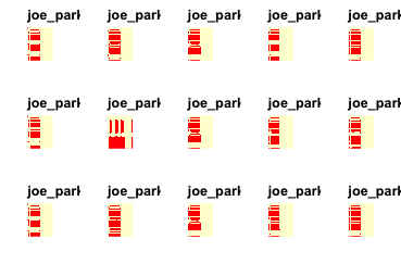
These appear to be sheets dedicated to periodic “Estimates” with a copy and pasted worksheet style. We are also likely to see the evolution of workbooks through time and their worksheets therein which results in a lack of diversity on our worksheets and t-SNE clustering those worksheets which are directly related. This is not useful, as this is just repeating the information found in the worksheet name. We could try this again after removing duplicate sheets (i.e. periodic accounting) which might result in more informative clusters based on the shape of a spreadsheet. t-SNE does not seem to be adding much value in this scenario as we might prefer to use our own spreadsheet experience to engineer better features rather than resorting to dimension reduction.
Another cluster
We repeat for another putative cluster.
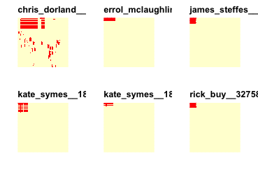
w <- which(tsne$Y[, 1] > 6 & tsne$Y[, 2] < 2)
w
paste("There are ", length(w), "worksheets in this range.")
## [1] 184 250 251## [1] "There are 3 worksheets in this range."But hide the code this time.
These are characterised by a top-leftedness, small and mostly empty. These are across a greater range of authors but captures their sameness.
This approach seems to be pretty good for identifying repeated structures or worksheets that are copy and pasted.
The other extreme
We look to the opposite end of the t-SNE plot and inspect those worksheets to get a feel for what these dimensions are capturing (third time I’ve done this, should of written a function).
w <- which(tsne$Y[, 1] < -7 & tsne$Y[, 2] < -10)
w
paste("There are ", length(w), "worksheets in this range.")
## [1] 10 72 76 110 111 201## [1] "There are 6 worksheets in this range."But hide the code this time.
Versioning spreadsheets retrospectively
This demonstrable clustering of spreadsheets around “evolutionary” groups was identified in our examples and by this paper and can be used to infer versioning of spreadsheets through time. It could also be helpful in identifying organisational risk as often errors creep in to his copy and pasting approach (16.9% of the time according to the cited paper (Liang et al., 2017)).
t-SNE extension
Given some labels for our spreadsheets, we could employ the same strategy used for the MNIST digit data set and described in our last blog post, where we use Support Vector Machines to train on our t-SNE’ed data.
Once I have a t-SNE map, how can I embed incoming test points in that map?
t-SNE learns a non-parametric mapping, which means that it does not learn an explicit function that maps data from the input space to the map (at least for now). Therefore, it is not possible to embed test points in an existing map (although you could re-run t-SNE on the full dataset). A potential approach to deal with this would be to train a multivariate regressor to predict the map location from the input data.
Feature engineering
Fortunately a recent literature review (Reschenhofer et al., 2017) provides a conceptual model for measuring the complexity of spreadsheets which might be useful in helping our classifying spreadsheets that are complex or not (although we lack this label on our Enron data), or in classifying the theme of a spreadsheet, or whether it’s tidy or not. We might expect, for example, any economic modelling spreadsheets to be more complicated than a spreadsheet for a social event (a list of names) which could be a useful predictor.
This model integrates knowledge about aspects for spreadsheet complexity based on existing complexity metrics. Interestingly these measures can be quantified and have origins in software development and linguistics. We summarise them here but see the paper for the full list:
Spreadsheet complexity Metrics
- Average abstract syntax tree (AST) depth per formula
- Number of formula cells
- Ratio of formula cells to non-empty cells
- Number of input cells (feed into a formula)
- Ratio of input cells to non-empty cells
- Ratio of formula cells to input cells
- Number of distinct formulas
- Average number of conditionals per formula
- Average spreading factor per formula
- Average number of functions per formula
- Average number of distinct functions per formula
- Average number of elements per formula
- Entropy of functions within a function
This review concluded with these aspects captured by the conceptual model for spreadsheet complexity being mostly independent from each other (through covariance of metrics), and a high complexity with respect to a certain aspect does not imply a high complexity with respect to another one. It would be interesting to explore the use of these metrics in feature engineering for our spreadsheets in an attempt to improve our classification of the theme of a spreadsheet. To achieve this we would need to read in and retain all the metadata stored about each cell rather than just the value of the cell.
Natural language processing (NLP) of content
Spreadsheet files are often designed to be informative in determining the theme and content therein. Some authors fail to give good names for files. A spreadsheet could contain worksheets of different themes. As well as numeric data and formulae, spreadsheets contain text to impart the theme or the context of the spreadsheet to the human reader. We could use NLP modelling with bag of words or bag of n-grams methods to facilitate a machine reading this content.
Deep learning
An alternative method that doesn’t rely on our manually selecting or feature engineering based on expert domain knowledge (which I don’t have) is to rely on deep learning (although we still need to help the process with a suitable abstraction; it’s not a free lunch). Deep learning has proven successful in image recognition, we could provide an abstraction of the spreadsheet structure that retains the visual and spatial structure.
We could implement the Melford method proposed in this paper (although again, where’s the code?). Essentially it recodes the contents of each cell by type (e.g. formula, empty, string, number). This can then be solved as a classification problem, whereby given the context of the surrounding cells what is the probability this specific cell contains an error based on sufficient training data.
We’re already part way there achieving this based on Duncan’s original preparation of the spreadsheet data demonstrated in the view_ranges object. However, we lack the important variable to train on, the presence or absence of an error. Thus we would need an unsupervised method for identifying cells which are unexpected (e.g. a harded coded number in a row full of formulas; the column totals). Given the training data what is the probability this cell has this type of data in it given it’s neighbours? If that probability were low then it suggests our cell has an unusual data type given its neighbours and would warrant inspection from a human. We wonder how different / better this approach is to the logic already implemented in a spreadsheet’s built-in error checking tools.
Closed source
Working in the spreadsheet domain is frustrating, presumably due to commercial interests, code is rarely openly available. This makes reproducing alot of the work and hype in these papers difficult.
Make things open, it makes things better.
Take home message
We applied our previous learning of converting an image of a digit into a matrix to the Enron spreadsheet data set. We used purrr and tidyxl to read in many worksheets from many workbooks. We decided on a sensible view range through data exploration of what was typical for an Enron spreadsheet. We then converted the existing matrix structure of a spreadsheet to a square matrix with 0 for empty cells and 1 for those with content. We then explored these data using visualisation. We extended the t-SNE method to this data set, with a larger matrix for every worksheet. This unsupervised approach seemed promising for separating out similar worksheets into clusters, however the problem was somewhat contrived t-SNE components probably not that useful as features, depending on the problem.
Given appropriate labels (e.g. tidy data or not) for a specific data science problem one could build on this approach to predict labels. This could be complemented by further feature engineering for each worksheet based on the literature and the problem domain. This would be a suitable route for automation given many organisations have huge numbers of spreadsheets in their knowledge repository. We also consider the use of deep learning which could be viable given a training set of thousands of sheets.
Acknowledgements
This project was inspired by Duncan Garmonsway and was undertaken using our development time at GDS.
Used a data-set and code to read in from this repo.
References
- Adelfio and Semet, 2013. The paper
- Chen and Caferella, 2013. The paper.
- EUSES corpus.
- Hermanns, 2015. The paper.
- Hermanns, 2015. Enron spreadsheet data.
- Liang Xu, Wensheng Dou, Chushu Gao, Jie Wang, Jun Wei, Hua Zhong, Tao Huang. SpreadCluster: Recovering Versioned Spreadsheets through Similarity-Based Clustering. In Proceedings of the 14th International Conference on Mining Software Repositories (MSR 2017), pages 158-169, Buenos Aires, Argentina, May 2017.
- Reschenofer et al., 2017. A Conceptual model for measuring the complexity of spreadsheets.
sessionInfo()## R version 3.4.1 (2017-06-30)
## Platform: x86_64-apple-darwin15.6.0 (64-bit)
## Running under: OS X El Capitan 10.11.6
##
## Matrix products: default
## BLAS: /System/Library/Frameworks/Accelerate.framework/Versions/A/Frameworks/vecLib.framework/Versions/A/libBLAS.dylib
## LAPACK: /Library/Frameworks/R.framework/Versions/3.4/Resources/lib/libRlapack.dylib
##
## locale:
## [1] en_GB.UTF-8/en_GB.UTF-8/en_GB.UTF-8/C/en_GB.UTF-8/en_GB.UTF-8
##
## attached base packages:
## [1] stats graphics grDevices utils datasets methods base
##
## other attached packages:
## [1] tidyr_0.6.3 openxlsx_4.0.17 e1071_1.6-8 Rtsne_0.13
## [5] bindrcpp_0.2 bayesAB_0.7.0 Matrix_1.2-10 ggplot2_2.2.1
## [9] simecol_0.8-7 deSolve_1.14 readxl_1.0.0 here_0.1
## [13] tidyxl_1.0.0 purrr_0.2.3 dplyr_0.7.3
##
## loaded via a namespace (and not attached):
## [1] Rcpp_0.12.14 highr_0.6 cellranger_1.1.0 compiler_3.4.1
## [5] plyr_1.8.4 bindr_0.1 class_7.3-14 tools_3.4.1
## [9] digest_0.6.12 evaluate_0.10 tibble_1.3.4 gtable_0.2.0
## [13] lattice_0.20-35 pkgconfig_2.0.1 rlang_0.1.2 yaml_2.1.14
## [17] stringr_1.2.0 knitr_1.16 rprojroot_1.2 grid_3.4.1
## [21] glue_1.1.1 R6_2.2.2 minqa_1.2.4 magrittr_1.5
## [25] codetools_0.2-15 backports_1.1.0 scales_0.4.1 assertthat_0.2.0
## [29] checkpoint_0.4.0 rmd2md_0.1.1 colorspace_1.3-2 stringi_1.1.5
## [33] lazyeval_0.2.0 munsell_0.4.3